
In this post, I discuss issues and possible avenues for grinding finer for filter coffee
Measuring Brew Water Properties

This post describes some available tools for measuring water properties relevant to coffee and presents ways and a web tool to hack aquarium kits for a better precision.
The Physics of Fines Migration

In this post, I explore the details of physical phenomena that can cause fines to migrate and clog coffee filters.
The Struggle for a Steady Kettle Flow
In this post I discuss recent developments in my efforts to stabilize my kettle flow rate.
The Hardness of Green Coffee
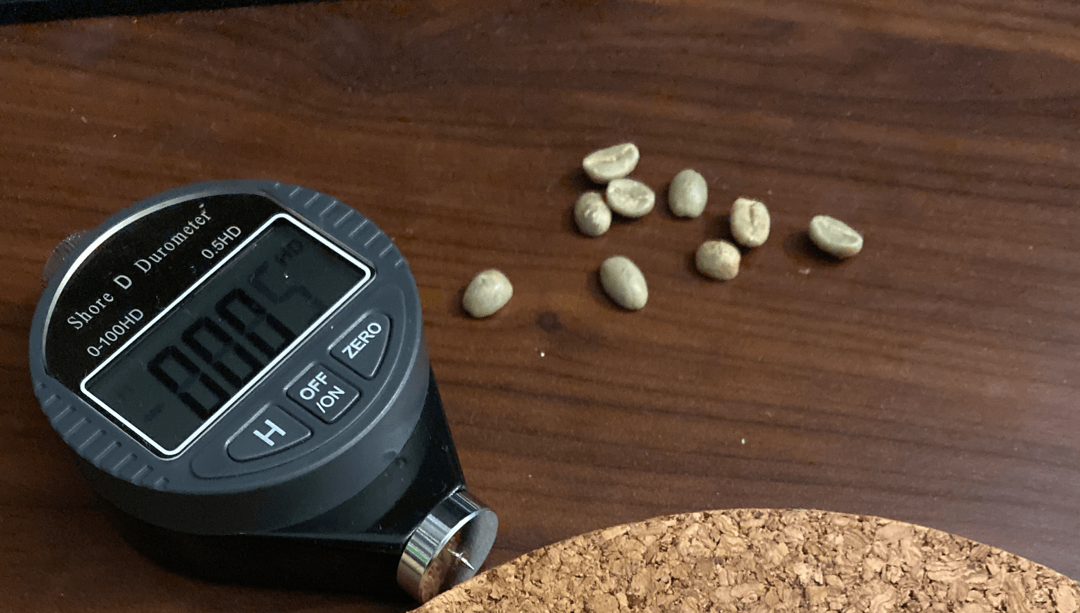
In this post, I show that surface hardness might vary more than mass density across different green coffees.
What is Astringency ?

In this post I describe what causes astringency, and talk about ideas how we could potentially measure it or remove it post brewing.
What Affects Brew Time

In this post I discuss the variables that affect brew time in detail
Extraction Uniformity and Channeling

For a while now I’ve been trying to understand the details of channeling in pour over coffee, and I found it very difficult to find a convincing description of why channeling (and thus astringency) happens suddenly when we grind a bit too fine, even if the surface of the coffee bed looks flat at theContinue reading "Extraction Uniformity and Channeling"
Measuring Coffee Concentration with a 0.01% Precision
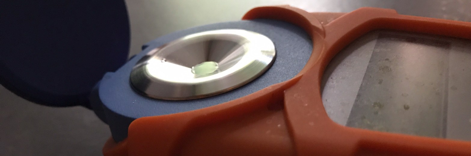
In this post I present an updated methodology to measure TDS with a 0.01% precision using a refractometer.
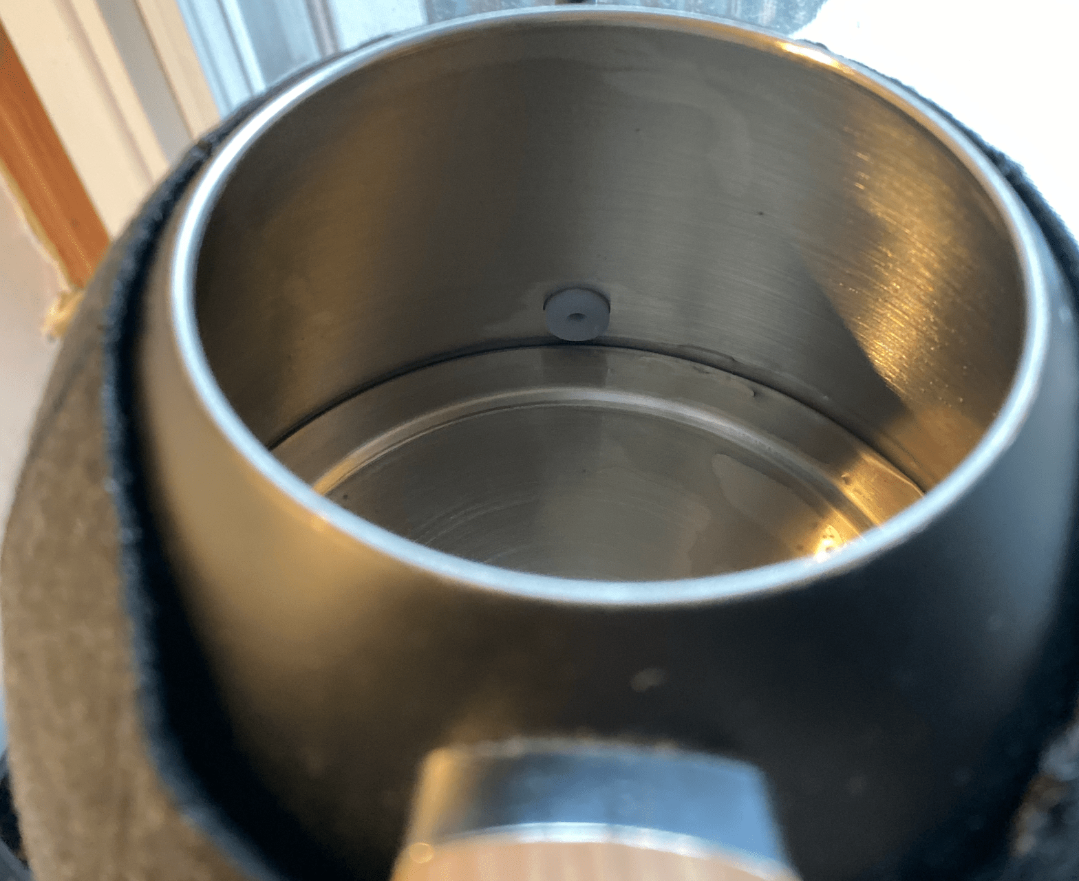
An Investigation of Kettle Temperature Stability

In this post I investigate the stability of my Brewista kettle with the Brewcoat insulation and an additional layer of aerogel.
